Geometallurgy

Geometallurgy is a python package that allows geoscientists and metallurgists to easily work with, and visualise mass-compositional data.

Geoscientific disciples, like Metallurgy, Geometallurgy, Geology, and Mining Engineering, rely on the analysis of data based on mass, moisture and chemistry. The data is collected from drill-holes, samples, and process streams. The data is used to model the behaviour of the material in the ground, and the material as it is processed.

The Geometallurgy package supports the geometallurgical workflow from drill-hole planning and data analysis, sample fractionation and mass balanced process simulation, through to 3D block model visualisation. The is designed to handle large datasets and provide the necessary visualisations to support the workflow. Plots are generally interactive to maximise context and insight. Assurance of data integrity is a key objective.

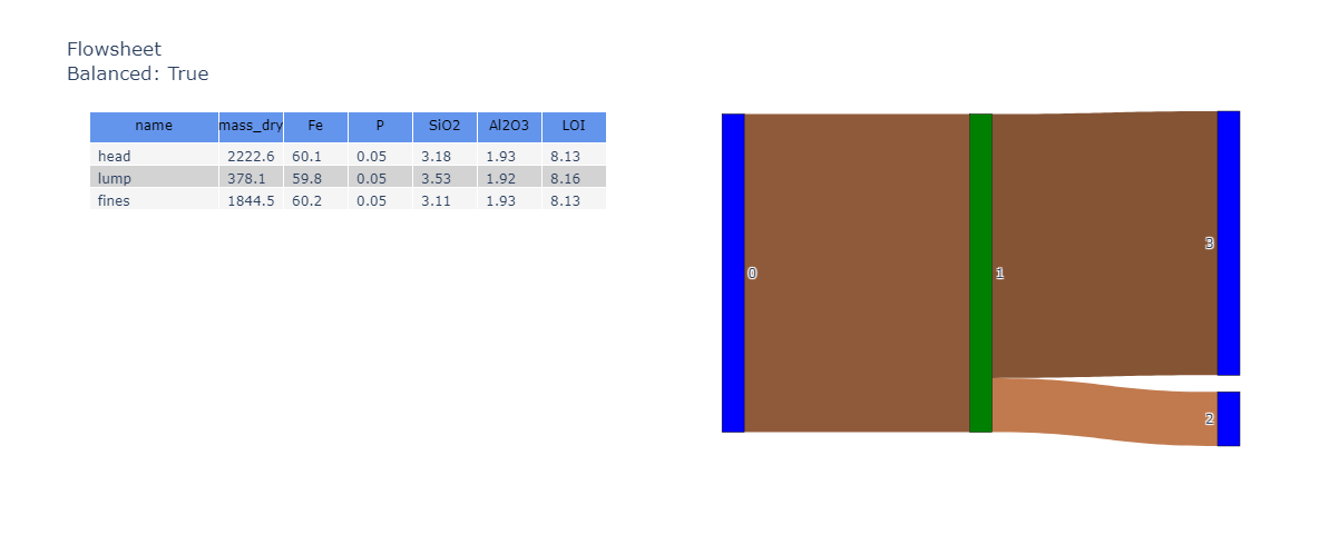
The package not only supports individual Samples, but collections of objects that are mathematically related in a Directional Graph (a.k.a. network or flowsheet).

This package is a rewrite of the mass-composition package (based on pandas only instead of pandas/xarray).

Prerequisites

Before you begin, ensure you have met the following requirements:

• You have installed the latest version of the mass-composition python package.
• You have a Windows/Linux/Mac machine.
• You have read the docs.

Installing Geometallurgy

To install Geometallurgy, follow these steps:

pip install geometallurgy

Or, if poetry is more your flavour.

poetry add "geometallurgy"

Using Geometallurgy

To use GeoMetallurgy to create a Sample object, follow these steps:

There are some basic requirements that the incoming DataFrame must meet. We'll use a sample DataFrame here.

df_data = sample_data()

Create the object

sample = Sample(df_data)

It is then trivial to calculate the weight average aggregate of the dataset.

sample.aggregate()

Multiple composition analytes can be viewed in a single interactive parallel coordinates plot.

sample = Sample(df_data.reset_index().set_index(['DHID', 'interval_from', 'interval_to']),
                name=name)

fig = sample.plot_parallel(color='Fe')
fig

Network visualisations and other plots are interactive.

For full examples, see the gallery.

License

This project uses the following license: MIT.